VLOOKUP, XLOOKUP and SUMIFS in a JavaScript spreadsheet

Every business sheet eventually grows the same pair of columns. One looks something up — a product code becomes a name and a unit price. The other adds things up, but only some of them — this category, those months, orders above a threshold. Between them they account for most of the formulas anyone actually writes.

Neither is hard in Excel. The question is what happens when the sheet moves into a browser, and whether you end up reimplementing lookup joins and conditional sums in application code because the grid underneath is only a grid.

This article builds one small order sheet in ReoGrid Web that does both in formulas, and is honest about the two lookup functions the engine does not have.

The formula engine has 109 built-in functions, and they ship in Pro. The free Lite tier evaluates arithmetic, comparisons and cell references — including the dependency graph and the colour-coded formula editor — but registers no named functions, so =SUM(...) there returns #NAME?. Everything below imports @reogrid/pro.

The sheet

Two blocks on one sheet. On the right, a product master: code, name, unit price, category. On the left, the order lines, where only the code and the quantity are typed — every other column is a formula. Underneath, a summary that rolls the lines up by category.

Result

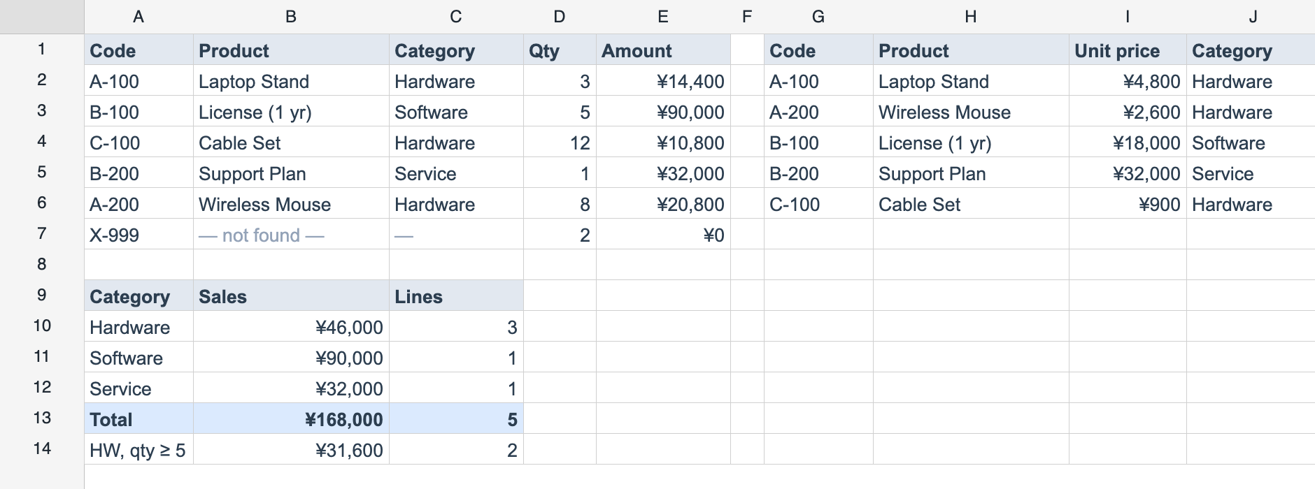
Here is the master, which is just data:

import { createReogrid } from '@reogrid/pro';

const grid = createReogrid({ workspace: '#grid', licenseKey: 'YOUR_LICENSE_KEY' });
const ws = grid.worksheet;

ws.suspendRender();
ws.setGridSize(14, 10);   // A..J — the default sheet is only 40 rows

const MASTER: Array<[string, string, number, string]> = [
  ['A-100', 'Laptop Stand',   4800,  'Hardware'],
  ['A-200', 'Wireless Mouse', 2600,  'Hardware'],
  ['B-100', 'License (1 yr)', 18000, 'Software'],
  ['B-200', 'Support Plan',   32000, 'Service'],
  ['C-100', 'Cable Set',      900,   'Hardware'],
];

['Code', 'Product', 'Unit price', 'Category'].forEach((h, i) =>
  ws.cell(0, 6 + i).setValue(h).setStyle({ bold: true, backgroundColor: '#e2e8f0' }));

MASTER.forEach(([code, name, price, category], r) => {
  ws.cell(1 + r, 6).setValue(code);
  ws.cell(1 + r, 7).setValue(name);
  ws.setCellInput(1 + r, 8, String(price));
  ws.cell(1 + r, 9).setValue(category);
});

ws.range('I2:I6').setFormat('¥#,##0');

setGridSize is worth a moment. A new sheet is 40 rows by 26 columns, and a range reaching past that edge is silently ignored rather than refused — so a master written into row 60 of a default sheet simply isn’t there, with nothing thrown to tell you. Size the sheet before you fill it.

VLOOKUP, and its two problems

VLOOKUP(value, table, col_index, [approx]) searches the first column of table and returns the value col_index columns to the right:

ws.setCellInput(1, 1, '=VLOOKUP($A2,$G$2:$J$6,2,FALSE)');   // name     → Laptop Stand
ws.setCellInput(1, 2, '=VLOOKUP($A2,$G$2:$J$6,4,FALSE)');   // category → Hardware

That works, and for a table you control it is perfectly reasonable. Two things about it age badly.

The first is col_index. It is a position, counted from the left edge of the range, so the formula encodes the master’s current column order. Insert a column into the master — a supplier, a tax class — and every VLOOKUP pointing past it returns the wrong field. Nothing errors; the numbers just quietly change.

The second is the fourth argument. Omit it and you get approximate match, which assumes the first column is sorted ascending and returns the largest value not exceeding the lookup. On unsorted product codes that produces a plausible-looking wrong row. FALSE — exact match — is what you almost always want, and it is the one you can forget to type.

XLOOKUP

XLOOKUP takes the lookup column and the return column as two separate ranges, so there is no index to drift:

// XLOOKUP(lookup, lookup_array, return_array, [if_not_found], [match_mode], [search_mode])
ws.setCellInput(1, 1, '=XLOOKUP($A2,$G$2:$G$6,$H$2:$H$6,"— not found —")');
ws.setCellInput(1, 2, '=XLOOKUP($A2,$G$2:$G$6,$J$2:$J$6,"—")');

Three differences that matter in a sheet other people will edit:

• The return range is named, not counted. Insert a column between them and both ranges shift with it — the formula keeps meaning “the name column”.
• Exact match is the default. match_mode 0 is assumed; -1 and 1 fall back to the next smaller or larger value, and 2 enables wildcards. You opt in to fuzziness.
• The fourth argument is the miss handler. if_not_found returns whatever you pass instead of #N/A.

search_mode is there too — 1 first-to-last (default), -1 last-to-first, ±2 binary search on a sorted array. -1 is the useful one: against an append-only price history, it finds the most recent row.

The amount column multiplies the typed quantity by a looked-up price, defaulting to 0 so an unknown code contributes nothing rather than poisoning the total:

ws.setCellInput(1, 4, '=D2*XLOOKUP($A2,$G$2:$G$6,$I$2:$I$6,0)');

The codes that aren’t there

Row 7 of the sheet is X-999, deliberately absent from the master. That is not an edge case — it is a Tuesday, when someone pastes last quarter’s order lines and two SKUs have been retired.

if_not_found is the cheapest fix, and it is local to the lookup. When the formula is more than a bare lookup, wrap it instead:

// IFNA catches only #N/A — a genuine miss
ws.setCellInput(1, 4, '=IFNA(D2*XLOOKUP($A2,$G$2:$G$6,$I$2:$I$6),0)');

// IFERROR catches everything, including your own #VALUE! and #DIV/0!
ws.setCellInput(1, 4, '=IFERROR(D2*XLOOKUP($A2,$G$2:$G$6,$I$2:$I$6),0)');

Prefer IFNA. IFERROR is the bigger hammer and it swallows the bugs you wanted to see — a #VALUE! from a text quantity is information, not noise. If you need to branch on the failure rather than replace it, ISNA, ISERR and ISERROR are all registered, and ERROR.TYPE gives you the numeric code.

Adding up only some of the rows

With every line priced, the summary is conditional aggregation. The single-criterion forms take the range being tested first:

// SUMIF(range, criteria, [sum_range]) — test column C, add up column E
ws.setCellInput(9, 1, '=SUMIF($C$2:$C$7,$A10,$E$2:$E$7)');
ws.setCellInput(9, 2, '=COUNTIF($C$2:$C$7,$A10)');

The *IFS forms reverse the order — the range being aggregated comes first, then range/criteria pairs:

// SUMIFS(sum_range, range1, criteria1, ...) — hardware, five units or more
ws.setCellInput(13, 1, '=SUMIFS($E$2:$E$7,$C$2:$C$7,"Hardware",$D$2:$D$7,">=5")');
ws.setCellInput(13, 2, '=COUNTIFS($C$2:$C$7,"Hardware",$D$2:$D$7,">=5")');

That argument-order flip between SUMIF and SUMIFS is Excel’s, not ours, and it is the single most common reason one of these returns 0 for no apparent reason. AVERAGEIF and AVERAGEIFS follow the same split.

Criteria syntax

A criterion is a value or a string carrying its own operator:

The comparison lives inside the string, which is why a criterion built at runtime is just concatenation — '">=" & F1' in a formula, or an ordinary template literal on the JavaScript side.

Why any of this beats doing it in JavaScript

You could compute all of it in application code and write finished numbers into the cells. The difference shows up on the first edit.

Dependencies are tracked as formulas are parsed, so changing a cell recalculates everything downstream of it — and only that:

ws.cell('I4').value = '19800';   // License: ¥18,000 → ¥19,800
// E3 recalculates, the Software row of the summary follows, the total follows

Correct a price in the master and the line amounts, the category subtotals and the grand total all move, in that order, without a re-render pass of your own. The same holds when a user types into the master — which is the whole point of shipping a spreadsheet rather than a table.

After a bulk load that bypassed the normal input path, rebuild the graph once:

ws.rebuildFormulas();

Formulas are also what survives the round trip. Export this sheet with ws.saveAsXlsx() and the recipient opens real XLOOKUP and SUMIFS formulas in Excel, still live. Precomputed values arrive as a dead grid of numbers.

What isn’t there

Two functions in the lookup family are not implemented: INDIRECT and OFFSET. Both build a reference at evaluation time, which means the dependency graph cannot know what a formula reads until it runs — volatile cells, in Excel’s terms. Supporting them properly is a change to the graph rather than a function to add, and it is planned rather than done.

In practice:

• INDIRECT is usually a dynamic sheet or range name. Compose the formula string in JavaScript and set it with setCellInput — you have a real programming language on the outside of the sheet, which is the thing INDIRECT was working around.
• OFFSET is usually a moving window. INDEX is registered, does not need volatility, and expresses the same thing: =INDEX($E$2:$E$100,$F$1) for a shifting row.

One smaller gap: single-cell ROW(A5) returns #VALUE!. Argument-less ROW() and COLUMN() work, and so do range arguments — ROWS($A$2:$A$7) for a row count is the idiom that behaves.

Also worth stating plainly: there is no public API for registering your own formula functions in ReoGrid Web. Custom functions are a ReoGrid .NET feature. On the web the extension point is the other direction — read and write cells from JavaScript, where you already have every library you want.

Wrapping up

The two columns this article started with are the ones that decide whether a browser sheet is a spreadsheet or a table with an Excel skin. Lookups make a code mean something; conditional aggregation makes a hundred rows mean something. Both belong in cells, attached to the data, recalculating when someone edits — not in a useEffect that has to remember to run.

Start with the formula engine documentation for the full list of all 109 functions and the criteria reference. From here, cross-sheet formulas move the master onto its own sheet where it belongs, pivot tables take over when the summary needs to be cross-tabbed rather than listed, and data validation stops the unknown product code from being typed in the first place.